Real-time recommendation models - part II.
Session-based approach in the real world
- Lukáš Matějka
![Lukáš Matějka]()
- 11 min read

In part I we have first outlined the basic concepts of recommendation systems and then focused mainly on the theory of session-based approach that is very useful for example in cases of missing historical data (typically happens when new customers visiting the web) — also known as so-called “cold start problem” or as a part of any recommendation engine in general because current customer’s behavior can better reflect their actual needs.
This part will be more practical, we are going to show which session-based models should be selected specifically for your client’s needs together with an explanation of why.
To be more concrete, this article will show you an experiment with three completely different datasets (two public and one private used by one of our clients) that should help to answer these questions. There are some data concessions used to make the experiment more demonstrative and therefore the results are confirming the used data cleaning, preprocessing, parameters, etc., clearly, we could reach better (or even different) results in a different setup. Also, some variables were completely missing in chosen public datasets so they were created on purpose (for example session ids).
Which session-based model to select?
As mentioned previously, it is always important to select the most appropriate model/algorithm/approach based on your data or client’s business use case. Each has its specific needs.
Used models
In this experiment we are going to challenge each other with the following session-based models whose theory was described in detail in the previous article:
- Rule-based models: Markow chain (MC), sequential rules (SR)
- KNN models: i-KNN (IKNN), session-KNN (SKNN), vector multiplication session-KNN (VKNN)
- RNN models: Gru4rec
- NLP models: session-based word2vec (w2v)*
- Baseline: random
*Word2Vec model wasn´t a part of the mentioned article, but it also can be a very good competitor on the field of session-based algorithms. If you would like to know more about it, I would recommend for example this article with basic usage.
Datasets Description
As an example, here we are focusing on three completely different datasets:
- Yoochoose: This is one of the datasets that was used in [Hidasi et al. 2016a] and their later works. It was published in the context of the ACM RecSys 2015 Challenge and contains recorded click sequences (item views, purchases) for a period of six months.
- Tmall: containing classical e-shop data. Tmall is a Chinese online retail e-shop selling brand-name goods. You can find there almost everything from clothes to electronics, food, or even cars. The dataset we are using was originally downloaded from this page. The dataset was published in the context of the Tmall competition and contains interaction logs of this e-shop.
- Product comparator: e-commerce product comparison site. Data are different from a classical e-shop because the majority of customers are non-returning. And if it happens that they come back, they probably go to find and compare absolutely different product(s) so to use learned history would be completely useless in this case.
Interactions
In this experiment we work only with one interaction type and that is the item view. In general, the most important interaction would be the purchase of an item (considering e-shops) describing the real customer´s intent. But this is irrelevant for the third dataset (so we would be unable to compare them, have rules from models, etc.). Secondly, there are usually not enough of such kinds of interactions from which session-based models could learn. Of course, there are a few other options (e.g. use more event types with various weights), however, this is not the aim of this article.
Below, you can find a 14-day timeframe of interactions collection demonstrating the difference in counts of each interaction type. Results were calculated using the first dataset.
Event counts during time period
Datasets explorations
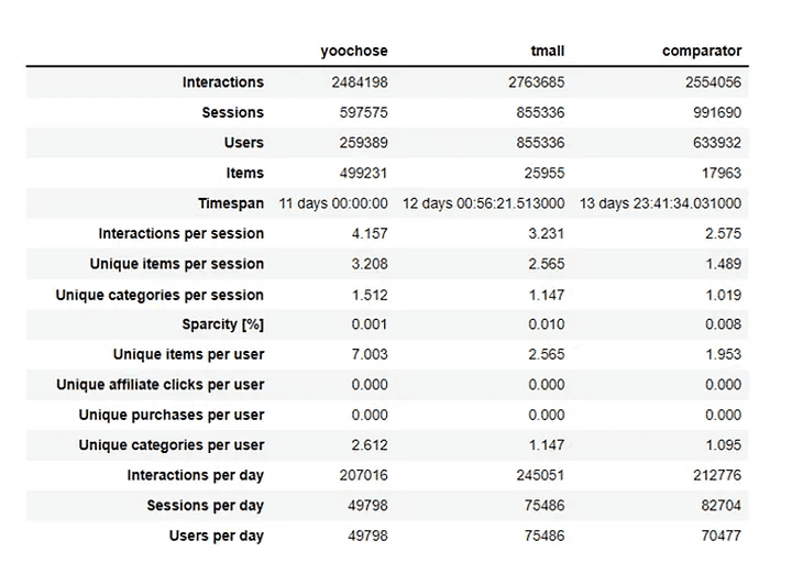
Comparison of chosen three datasets based on their basic web statistics. Simple average was used for every per* statistic.
All three datasets seem to have enough interactions (in this case item view) on the web so should be a good source for our experiment. And yoochoose dataset would probably be the best source of data for any session-based model because of the highest number of items per session together with the highest number of interactions per session. Notice also the ratio of items and users — evidentially for yoochoose there are twice more items than users. This can be tricky for any collaborative recommendation algorithms because of many so-called long-tail items — many items with no interaction so any model cannot know how to behave to these (see later section for more info).
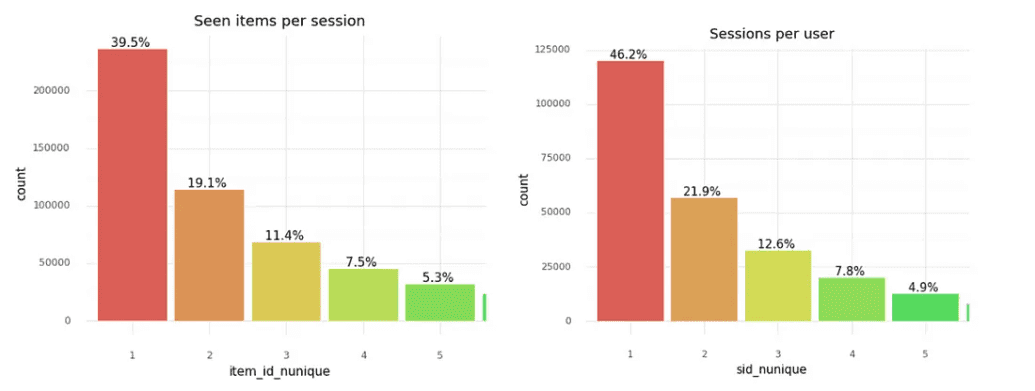
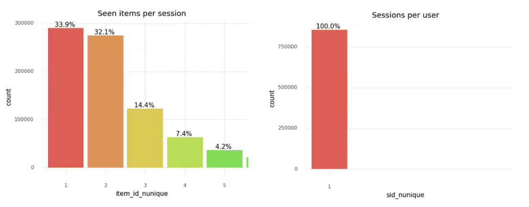
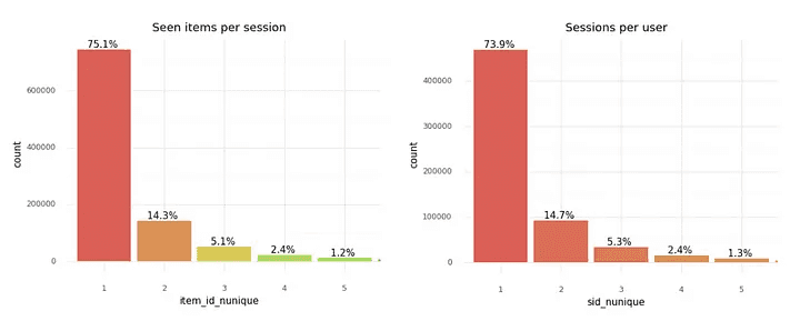
Below you can find deeper insight into each of datasets — distribution of seen items per session and sessions per user where the session is defined as (consequent interactions with a delay no longer than 30 minutes).
Yoochoose: Bar plots with number of seen items per session and count of sessions per user
Tmall: Bar plots with number of seen items per session and count of sessions per user
Comparator: Bar plots with number of seen items per session and count of sessions per user
We can notice some differences. Bar plots show that only yoochoose dataset is quite well-balanced. The others miss returning users (Tmall) or have a low number of items per session (comparator).
In the case of the comparator dataset, it would be quite hard for any kind of session-based model to learn something from such data — in one session there is mostly only one product so no rule can be extracted here and this part of data is completely useless at least for sequential rules algorithms. And together with only around 24% of users visiting the web more than once we do not have enough information either for KNN session-based models.
When considering both public datasets, the situation might be easier for all session-based models as more than 60% of sessions in the train dataset would contain at least two items from which models can be trained.
Models Comparison
Let’s see how each model will perform. Note — all models below are sorted according to cum_hit_rate@10 so it is easier to read from all plots at the same time.
Yoochoose
Metrics comparison (Yoochoose dataset)
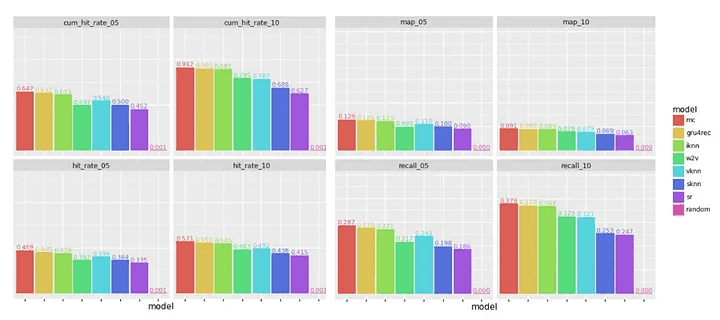
For yoochoose dataset it seems that the best session-based models with respect to accuracy metrics are: Markow Chain and Gru4Rec or IKNN model with hit_rate@10 over 0.5 which means that on average in 50% of cases, these models are recommended at least one item correctly when recommending 10 items. The same we can see on graphs with recall and map metrics.
Metrics comparison — arhr@k, mrr@k (Yoochoose dataset)
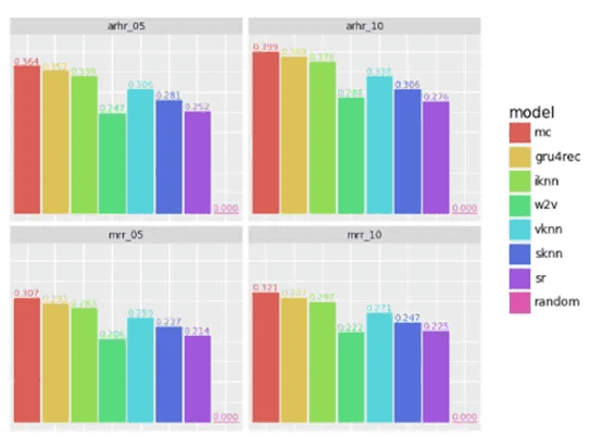
If we have a look at ranking metrics — you can notice that the „winner“ is again MC model and it does not matter if we do recommend 3, 5, 10, or even 25 items. In general, this model was able to recommend more than one-third of accurate positions on average.
And because mrr@k metrics values are almost the same as for arhr@k it basically signifies that really only 1 item on average was recommended correctly. If there was more than one correctly recommended item then arhr@k should be higher than mrr@k.
Now let’s have a deeper look at some of the so-called beyond-accuracy metrics. Would MC or Gru4rec still be winning?
Metrics comparison — price_ratio@k, coverage@k (Yoochoose dataset)
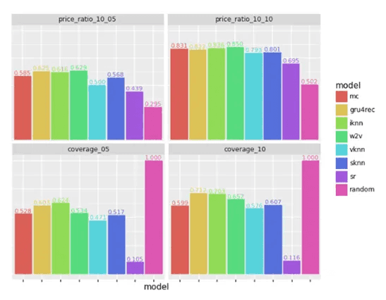
When looking at coverage — the absolute winner is of course the random model as it recommends randomly all the items from the item set. Then here Gru4Rec is definitely one-half of one-tenth better than MC model — this can be explained easily — MC model learns rules only from straightly consequently seen items which are definitely the smaller base of items overall than in the case of Gru4rec model. However, it is important to say that it does not necessarily denote that Gru4Rec is better, it is always crucial to take into consideration all the known metrics and if based on ranking and accuracy model A is better than B (even though B shows better results for example in coverage metric) then it only means that model B gives recommendation from more variety items dataset on the other hand but the final recommendation is found as a result with less success with the target customer. Similarly, Gru4rec, can be a bit better in terms of similar price per recommended items (at least in case of 10 recommendations) — price_ratio_10_10. This last resolution always depends on the recommendation scenario.
There is also another perspective — companies would like to recommend more variable items also from the so-called long-tail because, in the long-term perspective, it can bring better financial results (more on this topic below). That is why you need to take into consideration the difference between the first and second model in terms of accuracy metrics as well as the same in terms of beyond-accuracy metrics.
Hence, the final resolution for this dataset would be MC model in case we care only for short-term results but definitely Gru4rec model would be better in general.
Tmall
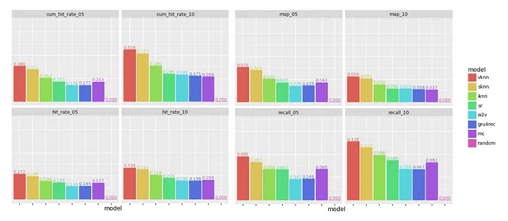
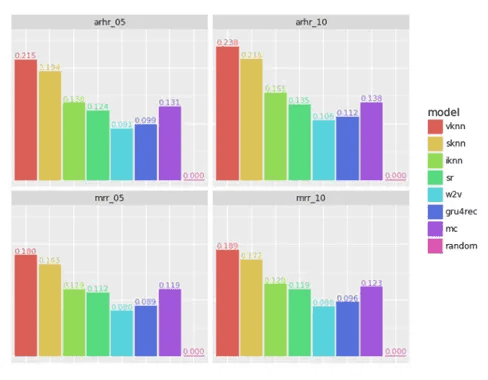
In this dataset, as expected, the situation is quite different — top models based on accuracy metrics (see attached plots) are all KNN models — and the absolute winner seems to be VKNN model which is a version of SKNN model, the only difference is more emphasis on the more recent events of a session in the process of computing the similarities. The same applies to recall@k and map@k metrics as can be seen below.
Metrics comparison (Tmall dataset)
Considering ranking metrics: the winners are still KNN models, however, MC is almost the same good as the worst KNN -> IKNN model.
Metrics comparison — arhr@k, mrr@k (Tmall dataset)
Secondly, as expected — SR has greater coverage than MC, also SR is better in ranking so in this case the first position in the case of hit rate metrics does not have such value.
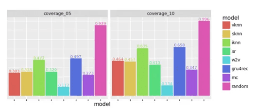
Metrics comparision — coverage@k (Tmall dataset)
Note, because of the not-present price for this dataset we cannot calculate the price_ratio@k metric.
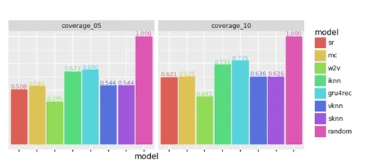
The highest coverage has by no surprise random model. From session-based models, the winners are IKNN and Gru4rec models with more than 10% increase than VKNN and SKNN. Hence, because VKNN and SKNN models were much better in accuracy metrics then the final recommendation hybrid model should consist of KNN models as a session-based part and the coverage can be caught up by different recommendation algorithms.
Comparator
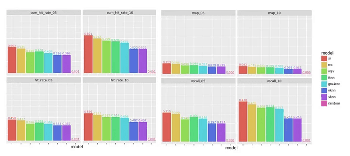
In case of the last dataset, based on hit rate metrics the absolute winner is SR model with more than 5% lead. It is a winner also when looking at map@k and recall@k. Anyway, it is surprising that so many good final metrics these session-based models have in the comparison to datasets description above. Probably, there are several customers who behave (watch products in some order) completely the same (in train and test dataset).
Metrics comparison (comparator dataset)
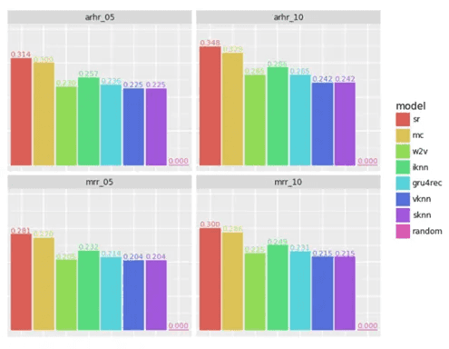
Nothing special happens in case of ranking metrics.
Metrics comparison — arhr@k, mrr@k (comparator dataset)
And as a last part, the highest coverage has (except random): Gru4rec and IKNN which is the same result as the previous dataset had. Evidentially, these two models work with a wider scale of products (by definition) but at a cost of lower accuracy and ranking precision.
And the final recommendation of which model to choose is also the same as in case of Tmall dataset — the difference between Gru4rec and SR on accuracy metrics is almost 20% (cum_hit_rate@10) which does not compensate the little bit “wider” item catalogue usage in recommendations.
Metrics comparison — coverage@k (comparator dataset)
Summary
The final overview of all datasets and best models can be seen in the table below. We can choose different candidates when considering short-term (e.g., instant sales boost) or long-term. Other aspects that need to be considered for proper choosing the most appropriate model is also computation feasibility (cpu and memory used by training and model runtime) and response speed. However, these aspects are not addressed in this article.
Final model selection overview
Long tail, short head
These two terms were firstly coined in a marketing field almost twenty years ago and now they are tightly connected with recommendations as well which you can notice in the previous section.
From the recommendation perspective, every item catalogue can be split into two main parts: short-head and long-tail products. Short head is composed of the most popular items that are often bought/viewed by customers (usually top 20%) and all other products belong to long tail. There is also the so-called long-tail concept focusing on selling less popular items with lower demand to increase the company´s profit as a result. One reason for that is the need for customers to navigate away from mainstream popular products.
Therefore, if the recommendation engine can work well with items from long tail or even advances them to the top positions, it can lead to greater customer satisfaction and then to higher revenue at the end from the long-term perspective.
Unfortunately, by default, all session-based models mentioned in this article learn the majority of rules from the short head (because the more the rule occurs in the training dataset the more it is weighted as a good rule which should be used for the recommendation). And that is why it is also crucial to evaluate both kinds of metrics: accuracy and beyond-accuracy — specifically the coverage rate in this case.
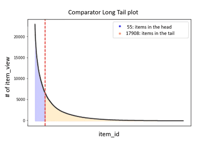
For our comparator dataset, the ratio of short-head and long-tail items are as follows in the attached Long Tail plot. Mostly 55 (0.3%) items would be recommended if we use only a session-based approach in the recommendation engine. And that can be quite unattractive after a really short period of time for all the customers plus then we can only hardly talk about a tailored recommendation to all the customers.
Short-head vs long tail (comparator dataset)
The rest of the 17.9K items would be used at rear recommendation positions or more likely the majority of them would have never ever been used because no rules with them were extracted.
To be more particular, imagine that you need to create a recommendation list of 10 items for a short-head item (A) in your catalogue. If the average of seen items per user is less than 2 (see section datasets description), then you need at least 10 users who saw item A together with another always different item. If we choose some item (B) from the long tail, the probability of finding all ten rules is almost equal to zero. Also, in the table below (representing the comparator dataset) there are 6% of items that were in less than 10 interactions from the whole 2.5M so for these items it is impossible to find 10 other items to be recommended by any default session-based algorithm.
interactions frequencies
To sum it up
We could see one from many ways how to select the best fitting model for the selected dataset. Evidently, every e-commerce company has different data based on its own customers and business specifics, therefore some session-based models work better than others.
We could also notice that companies with smaller product catalogues but larger user bases probably should profit from sequential rules models whereas in the opposite case, KNN models seem to be more appropriate.
What is important, in some cases session-based models might be the best and only option for your recommendation task or business. But in many real situations, you need to select a hybrid approach and add additional recommendation layers in order to create relevant recommendations. For example, selecting products from long-tail, and in general to make the recommendation list more variable (and probably more attractive for your customers). The easiest way is to add for instance so-called simple popularity model, which extracts as its name suggests, the most popular items from the whole item catalogue (= items with the most interactions) which do not suffer from doing recommendation which gets along with currently viewed item on the page or in cases of a completely new customer who hasn´t seen anything on the webpage yet. But be sure that such layer won’t help you with the broadening of long-tail products.
In every case, be aware that once you combine session-based models with any other model kind then it does not necessarily mean that if for example best-shown model was Markow chain then the combination of MC and for example mentioned popularity model would work better than the popularity model with IKNN model. The final combination of resulting items may be differently good so you always have to do a new evaluation. And last but not least, accuracy and beyond-accuracy metrics are very important together but if you want to have a superior recommendation engine then we suggest also doing so-called qualitative analysis on top of quantitative one and check results also by annotators (e.g. using annotator agreement).
Thanks also to co-author ❤️ Simona Navrátilová.
Did you have fun reading it?
Let's talk about it more!
Prague
Aguan s.r.o.Kaprova 42/14110 00 PrahaCzech republicIN: 24173681+420 222 253 015info@lundegaard.eu
Prague
Lundegaard a.s.Futurama Business ParkSokolovská 651/136a186 00 Praha 8 - KarlínCzech republicIN: 25687221+420 222 253 015info@lundegaard.eu
Brno
Lundegaard a.s.Ponávka Business CentreŠkrobárenská 502/1617 00 Brno - jihCzech republicIN: 25687221+420 222 253 025info@lundegaard.eu
Hradec Králové
Lundegaard a.s.Velké náměstí 1/3500 03 Hradec KrálovéCzech republicIN: 25687221+420 222 253 015office.hradec-kralove@lundegaard.eu
All rights reserved by Lundegaard a.s.
Services provided by Aguan s.r.o.


